Bevezetés az R-be 2.0 - Feladatgyűjtemény

Ábrák

1. feladat. Egydimenziós pontdiagram.
Rajzoljunk egydimenziós pontdiagramot a MASS csomag survey adattáblájának Height oszlopára. Fokozatosan javítsuk, és tegyük publikációkésszé!

data(survey, package = "MASS") # a survey beolvasása
survey$Height

  [1] 173.00 177.80     NA 160.00 165.00 172.72 182.88 157.00 175.00 167.00 156.20     NA 155.00
 [14] 155.00     NA 156.00 157.00 182.88 190.50 177.00 190.50 180.34 180.34 184.00     NA     NA
 [27] 172.72 175.26     NA 167.00     NA 180.00 166.40 180.00     NA 190.00 168.00 182.50 185.00
 [40] 171.00 169.00 154.94 172.00 176.50 180.34 180.34 180.00 170.00 168.00 165.00 200.00 190.00
 [53] 170.18 179.00 182.00 171.00 157.48     NA 177.80 175.26 187.00 167.64 178.00 170.00 164.00
 [66] 183.00 172.00     NA 180.00     NA 170.00 176.00 171.00 167.64 165.00 170.00 165.00 165.10
 [79] 165.10 185.42     NA 176.50     NA     NA 167.64 167.00 162.56 170.00 179.00     NA 183.00
 [92]     NA 165.00 168.00 179.00     NA 190.00 166.50 165.00 175.26 187.00 170.00 159.00 175.00
[105] 163.00 170.00 172.00     NA 180.00 180.34 175.00 190.50 170.18 185.00 162.56 158.00 159.00
[118] 193.04 171.00 184.00     NA 177.00 172.00 180.00 175.26 180.34 172.72 178.50 157.00 152.00
[131] 187.96 178.00     NA 160.02 175.26 189.00 172.00 182.88 170.00 167.00 175.00 165.00 172.72
[144] 180.00 172.00 185.00 187.96 185.42 165.00 164.00 195.00 165.00 152.40 172.72 180.34 173.00
[157]     NA 167.64 187.96 187.00 167.00 168.00 191.80 169.20 177.00 168.00 170.00 160.02 189.00
[170] 180.34 168.00 182.88     NA 165.00 157.48 170.00 172.72 164.00     NA 162.56 172.00 165.10
[183] 162.50 170.00 175.00 168.00 163.00 165.00 173.00 196.00 179.10 180.00 176.00 160.02 157.48
[196] 165.00 170.18 154.94 170.00 164.00 167.00 174.00     NA 160.00 179.10 168.00 153.50 160.00
[209] 165.00 171.50 160.00 163.00     NA 165.00 168.90 170.00     NA 185.00 173.00 188.00 171.00
[222] 167.64 162.56 150.00     NA     NA 170.18 185.00 167.00 185.00 169.00 180.34 165.10 160.00
[235] 170.00 183.00 168.50

Kiinduló ábra

stripchart(survey$Height)

plot of chunk abrak_egydimpont_1

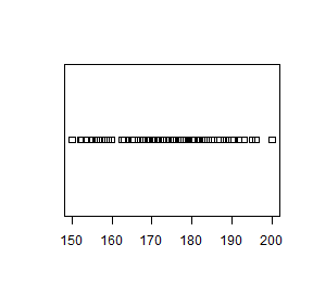
Legyenek kör alakú pontok!

stripchart(survey$Height, pch=1)

plot of chunk abrak_egydimpont_2

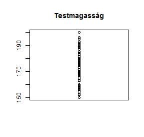
Függőleges pontsor

stripchart(survey$Height, pch=1, vertical=T)

plot of chunk abrak_egydimpont_3

Főcím hozzáadása

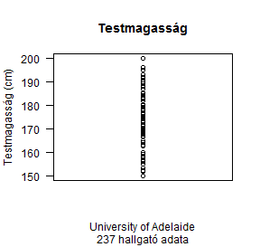
stripchart(survey$Height, pch=1, vertical=T, main="Testmagasság")

plot of chunk abrak_egydimpont_4

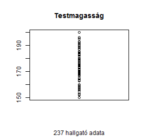
Alcím hozzáadása

stripchart(survey$Height, pch=1, vertical=T, main="Testmagasság", 
           sub="237 hallgató adata")

plot of chunk abrak_egydimpont_5

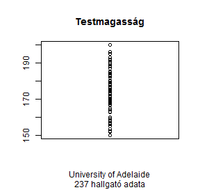
Az x tengely felirata

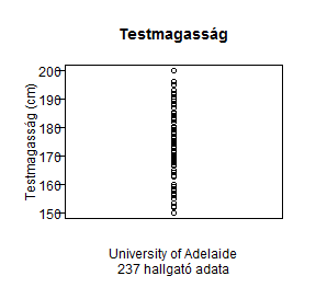
stripchart(survey$Height, pch=1, vertical=T, main="Testmagasság", 
           sub="237 hallgató adata", xlab="University of Adelaide")

plot of chunk abrak_egydimpont_6

Az y tengely felirata

stripchart(survey$Height, pch=1, vertical=T, main="Testmagasság", 
           sub="237 hallgató adata", xlab="University of Adelaide", ylab="Testmagasság (cm)")

plot of chunk abrak_egydimpont_7

Tengelyfeliratok írásirányának megfordítása

par(las=1)
stripchart(survey$Height, pch=1, vertical=T, main="Testmagasság", 
           sub="237 hallgató adata", xlab="University of Adelaide", ylab="Testmagasság (cm)")

plot of chunk abrak_egydimpont_8

Tengely és feliratok közelebb

par(las=1)
par(mgp=c(1.7, 0.2, 0))
stripchart(survey$Height, pch=1, vertical=T, main="Testmagasság", 
           sub="237 hallgató adata", xlab="University of Adelaide", ylab="Testmagasság (cm)")

plot of chunk abrak_egydimpont_9

Léptekjel mérete és iránya

par(las=1)
par(mgp=c(1.7, 0.2, 0))
par(tcl=-0.2)
stripchart(survey$Height, pch=1, vertical=T, main="Testmagasság", 
           sub="237 hallgató adata", xlab="University of Adelaide", ylab="Testmagasság (cm)")

plot of chunk abrak_egydimpont_10

Margók beállítása

par(las=1)
par(mgp=c(1.7, 0.2, 0))
par(tcl=-0.2)
par(mar=c(4.1, 3, 2, 1))
stripchart(survey$Height, pch=1, vertical=T, main="Testmagasság", 
           sub="237 hallgató adata", xlab="University of Adelaide", ylab="Testmagasság (cm)")

plot of chunk abrak_egydimpont_11

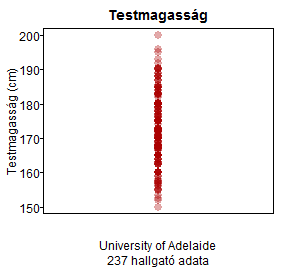
Pontkarakter beállítása, körvonal és kitöltés állítása

par(las=1)
par(mgp=c(1.7, 0.2, 0))
par(tcl=-0.2)
par(mar=c(4.1, 3, 2, 1))
stripchart(survey$Height, pch=21, vertical=T, main="Testmagasság", 
           sub="237 hallgató adata", xlab="University of Adelaide", 
           ylab="Testmagasság (cm)", col="#aa000010", bg="#aa000055", cex=1.5)

plot of chunk abrak_egydimpont_12

Betűtípus beállítása

windowsFonts(Times="Times New Roman")
par(family = "Times")
par(las=1)
par(mgp=c(1.7, 0.2, 0))
par(tcl=-0.2)
par(mar=c(4.1, 3, 2, 1))
stripchart(survey$Height, pch=21, vertical=T, main="Testmagasság", 
           sub="237 hallgató adata", xlab="University of Adelaide", 
           ylab="Testmagasság (cm)", col="#aa000010", bg="#aa000055", cex=1.5)

plot of chunk abrak_egydimpont_13

Betűméret beállítása

windowsFonts(Times="Times New Roman")
par(family = "Times")
par(las=1)
par(mgp=c(1.7, 0.2, 0))
par(tcl=-0.2)
par(mar=c(4.1, 3, 2, 1))
stripchart(survey$Height, pch=21, vertical=T, main="Testmagasság", 
           sub="237 hallgató adata", xlab="University of Adelaide", 
           ylab="Testmagasság (cm)", col="#aa000010", bg="#aa000055", 
           cex=1.5, cex.main=1.4, cex.sub=1.1, cex.lab=1.1, cex.axis=0.8)

plot of chunk abrak_egydimpont_14

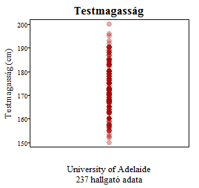
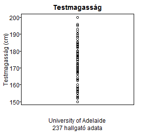
Ábrázolási mód változtatása: jitter

windowsFonts(Times="Times New Roman")
par(family = "Times")
par(las=1)
par(mgp=c(1.7, 0.2, 0))
par(tcl=-0.2)
par(mar=c(4.1, 3, 2, 1))
stripchart(survey$Height, pch=21, vertical=T, main="Testmagasság", 
           sub="237 hallgató adata", xlab="University of Adelaide", 
           ylab="Testmagasság (cm)", col="#aa000010", bg="#aa000055", 
           cex=1.5, cex.main=1.4, cex.sub=1.1, cex.lab=1.1, cex.axis=0.8, 
           method = "jitter")

plot of chunk abrak_egydimpont_15

Ábra mentése

# png("kepek/kep_stripchart.png", width=1200, height=1200, res=300)
# windowsFonts(Times="Times New Roman")
# par(family = "Times")
# par(las=1)
# par(mgp=c(1.7, 0.2, 0))
# par(tcl=-0.2)
# par(mar=c(4.1, 3, 2, 1))
# stripchart(survey$Height, pch=21, vertical=T, main="Testmagasság", sub="237 hallgató adata", xlab="University of Adelaide", ylab="Testmagasság (cm)", col="#aa000010", bg="#aa000055", cex=1.5, cex.main=1.4, cex.sub=1.1, cex.lab=1.1, cex.axis=0.8, method = "jitter") 
# dev.off()

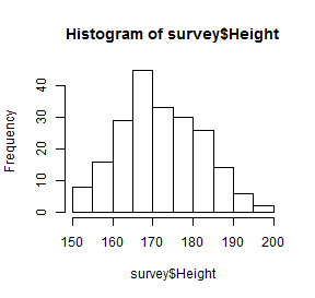
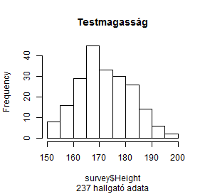
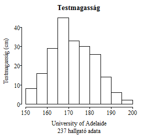
1. feladat. Hisztogram.
Rajzoljunk hisztogramot a MASS csomag survey adattáblájának Height oszlopára. Fokozatosan javítsuk, és tegyük publikációkésszé!

data(survey, package = "MASS") # a survey beolvasása
survey$Height

  [1] 173.00 177.80     NA 160.00 165.00 172.72 182.88 157.00 175.00 167.00 156.20     NA 155.00
 [14] 155.00     NA 156.00 157.00 182.88 190.50 177.00 190.50 180.34 180.34 184.00     NA     NA
 [27] 172.72 175.26     NA 167.00     NA 180.00 166.40 180.00     NA 190.00 168.00 182.50 185.00
 [40] 171.00 169.00 154.94 172.00 176.50 180.34 180.34 180.00 170.00 168.00 165.00 200.00 190.00
 [53] 170.18 179.00 182.00 171.00 157.48     NA 177.80 175.26 187.00 167.64 178.00 170.00 164.00
 [66] 183.00 172.00     NA 180.00     NA 170.00 176.00 171.00 167.64 165.00 170.00 165.00 165.10
 [79] 165.10 185.42     NA 176.50     NA     NA 167.64 167.00 162.56 170.00 179.00     NA 183.00
 [92]     NA 165.00 168.00 179.00     NA 190.00 166.50 165.00 175.26 187.00 170.00 159.00 175.00
[105] 163.00 170.00 172.00     NA 180.00 180.34 175.00 190.50 170.18 185.00 162.56 158.00 159.00
[118] 193.04 171.00 184.00     NA 177.00 172.00 180.00 175.26 180.34 172.72 178.50 157.00 152.00
[131] 187.96 178.00     NA 160.02 175.26 189.00 172.00 182.88 170.00 167.00 175.00 165.00 172.72
[144] 180.00 172.00 185.00 187.96 185.42 165.00 164.00 195.00 165.00 152.40 172.72 180.34 173.00
[157]     NA 167.64 187.96 187.00 167.00 168.00 191.80 169.20 177.00 168.00 170.00 160.02 189.00
[170] 180.34 168.00 182.88     NA 165.00 157.48 170.00 172.72 164.00     NA 162.56 172.00 165.10
[183] 162.50 170.00 175.00 168.00 163.00 165.00 173.00 196.00 179.10 180.00 176.00 160.02 157.48
[196] 165.00 170.18 154.94 170.00 164.00 167.00 174.00     NA 160.00 179.10 168.00 153.50 160.00
[209] 165.00 171.50 160.00 163.00     NA 165.00 168.90 170.00     NA 185.00 173.00 188.00 171.00
[222] 167.64 162.56 150.00     NA     NA 170.18 185.00 167.00 185.00 169.00 180.34 165.10 160.00
[235] 170.00 183.00 168.50

Kiinduló ábra

hist(survey$Height)

plot of chunk abrak_hisztogram_1

Főcím hozzáadása

hist(survey$Height, main="Testmagasság")

plot of chunk abrak_hisztogram_2

Alcím hozzáadása

hist(survey$Height, main="Testmagasság", sub="237 hallgató adata")

plot of chunk abrak_hisztogram_3

Az x tengely felirata

hist(survey$Height, main="Testmagasság", sub="237 hallgató adata", 
     xlab="University of Adelaide")

plot of chunk abrak_hisztogram_4

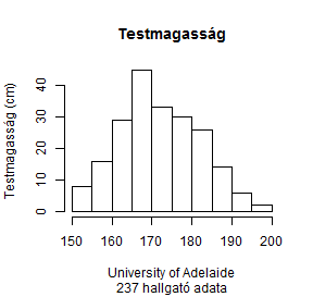
Az y tengely felirata

hist(survey$Height, main="Testmagasság", sub="237 hallgató adata", 
     xlab="University of Adelaide", ylab="Testmagasság (cm)")

plot of chunk abrak_hisztogram_5

Tengelyfeliratok írásirányának megfordítása

par(las=1)
hist(survey$Height, main="Testmagasság", sub="237 hallgató adata", 
     xlab="University of Adelaide", ylab="Testmagasság (cm)")

plot of chunk abrak_hisztogram_6

Tengely és feliratok közelebb

par(las=1)
par(mgp=c(1.7, 0.2, 0))
hist(survey$Height, main="Testmagasság", sub="237 hallgató adata", 
     xlab="University of Adelaide", ylab="Testmagasság (cm)")

plot of chunk abrak_hisztogram_7

Léptekjel mérete és iránya

par(las=1)
par(mgp=c(1.7, 0.2, 0))
par(tcl=-0.2)
hist(survey$Height, main="Testmagasság", sub="237 hallgató adata", 
     xlab="University of Adelaide", ylab="Testmagasság (cm)")

plot of chunk abrak_hisztogram_8

Margók beállítása

par(las=1)
par(mgp=c(1.7, 0.2, 0))
par(tcl=-0.2)
par(mar=c(4.1, 3, 2, 1))
hist(survey$Height, main="Testmagasság", sub="237 hallgató adata", 
     xlab="University of Adelaide", ylab="Testmagasság (cm)")

plot of chunk abrak_hisztogram_9

Betűtípus beállítása

windowsFonts(Times="Times New Roman")
par(family = "Times")
par(las=1)
par(mgp=c(1.7, 0.2, 0))
par(tcl=-0.2)
par(mar=c(4.1, 3, 2, 1))
hist(survey$Height, main="Testmagasság", sub="237 hallgató adata", 
     xlab="University of Adelaide", ylab="Testmagasság (cm)")

plot of chunk abrak_hisztogram_10

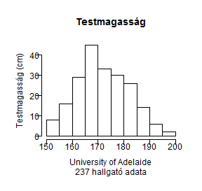
Betűméret beállítása

windowsFonts(Times="Times New Roman")
par(family = "Times")
par(las=1)
par(mgp=c(1.7, 0.2, 0))
par(tcl=-0.2)
par(mar=c(4.1, 3, 2, 1))
hist(survey$Height, main="Testmagasság", sub="237 hallgató adata", 
     xlab="University of Adelaide", ylab="Testmagasság (cm)", 
     cex.main=1.4, cex.sub=1.1, cex.lab=1.1, cex.axis=0.8)

plot of chunk abrak_hisztogram_11

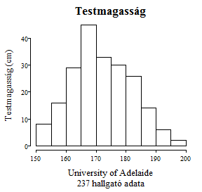
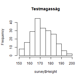
Oszlopszínek beállítása

windowsFonts(Times="Times New Roman")
par(family = "Times")
par(las=1)
par(mgp=c(1.7, 0.2, 0))
par(tcl=-0.2)
par(mar=c(4.1, 3, 2, 1))
hist(survey$Height, main="Testmagasság", sub="237 hallgató adata", 
     xlab="University of Adelaide", ylab="Testmagasság (cm)", 
     cex.main=1.4, cex.sub=1.1, cex.lab=1.1, cex.axis=0.8, col="seashell2")

plot of chunk abrak_hisztogram_12

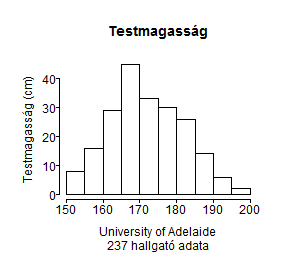
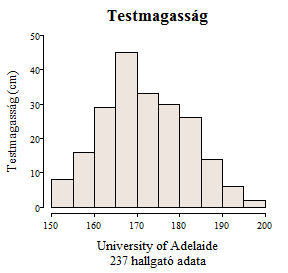
Az y tengely láthatósági tartománya

windowsFonts(Times="Times New Roman")
par(family = "Times")
par(las=1)
par(mgp=c(1.7, 0.2, 0))
par(tcl=-0.2)
par(mar=c(4.1, 3, 2, 1))
hist(survey$Height, main="Testmagasság", sub="237 hallgató adata", 
     xlab="University of Adelaide", ylab="Testmagasság (cm)", 
     cex.main=1.4, cex.sub=1.1, cex.lab=1.1, cex.axis=0.8, col="seashell2", ylim=c(0, 50))

plot of chunk abrak_hisztogram_13

Ábra mentése

# png("kepek/kep_hist.png", width=1200, height=1200, res=300)
# windowsFonts(Times="Times New Roman")
# par(family = "Times")
# par(las=1)
# par(mgp=c(1.7, 0.2, 0))
# par(tcl=-0.2)
# par(mar=c(4.1, 3, 2, 1))
# hist(survey$Height, main="Testmagasság", sub="237 hallgató adata", xlab="University of Adelaide", ylab="Testmagasság (cm)", cex.main=1.4, cex.sub=1.1, cex.lab=1.1, cex.axis=0.8, col="seashell2", ylim=c(0, 50)) 
# dev.off()

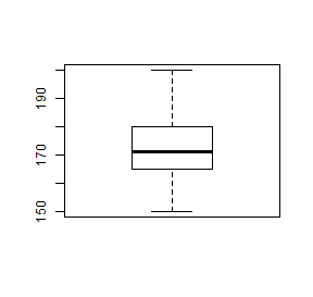
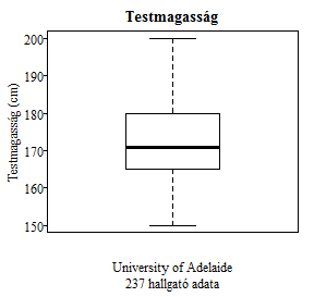
3. feladat. Dobozdiagram.
Rajzoljunk dobozdiagramot a MASS csomag survey adattáblájának Height oszlopára. Fokozatosan javítsuk, és tegyük publikációkésszé!

data(survey, package = "MASS") # a survey beolvasása
survey$Height

  [1] 173.00 177.80     NA 160.00 165.00 172.72 182.88 157.00 175.00 167.00 156.20     NA 155.00
 [14] 155.00     NA 156.00 157.00 182.88 190.50 177.00 190.50 180.34 180.34 184.00     NA     NA
 [27] 172.72 175.26     NA 167.00     NA 180.00 166.40 180.00     NA 190.00 168.00 182.50 185.00
 [40] 171.00 169.00 154.94 172.00 176.50 180.34 180.34 180.00 170.00 168.00 165.00 200.00 190.00
 [53] 170.18 179.00 182.00 171.00 157.48     NA 177.80 175.26 187.00 167.64 178.00 170.00 164.00
 [66] 183.00 172.00     NA 180.00     NA 170.00 176.00 171.00 167.64 165.00 170.00 165.00 165.10
 [79] 165.10 185.42     NA 176.50     NA     NA 167.64 167.00 162.56 170.00 179.00     NA 183.00
 [92]     NA 165.00 168.00 179.00     NA 190.00 166.50 165.00 175.26 187.00 170.00 159.00 175.00
[105] 163.00 170.00 172.00     NA 180.00 180.34 175.00 190.50 170.18 185.00 162.56 158.00 159.00
[118] 193.04 171.00 184.00     NA 177.00 172.00 180.00 175.26 180.34 172.72 178.50 157.00 152.00
[131] 187.96 178.00     NA 160.02 175.26 189.00 172.00 182.88 170.00 167.00 175.00 165.00 172.72
[144] 180.00 172.00 185.00 187.96 185.42 165.00 164.00 195.00 165.00 152.40 172.72 180.34 173.00
[157]     NA 167.64 187.96 187.00 167.00 168.00 191.80 169.20 177.00 168.00 170.00 160.02 189.00
[170] 180.34 168.00 182.88     NA 165.00 157.48 170.00 172.72 164.00     NA 162.56 172.00 165.10
[183] 162.50 170.00 175.00 168.00 163.00 165.00 173.00 196.00 179.10 180.00 176.00 160.02 157.48
[196] 165.00 170.18 154.94 170.00 164.00 167.00 174.00     NA 160.00 179.10 168.00 153.50 160.00
[209] 165.00 171.50 160.00 163.00     NA 165.00 168.90 170.00     NA 185.00 173.00 188.00 171.00
[222] 167.64 162.56 150.00     NA     NA 170.18 185.00 167.00 185.00 169.00 180.34 165.10 160.00
[235] 170.00 183.00 168.50

Kiinduló ábra

boxplot(survey$Height)

plot of chunk abrak_dobozdiagram_1

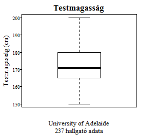
Főcím hozzáadása

boxplot(survey$Height, main="Testmagasság")

plot of chunk abrak_dobozdiagram_2

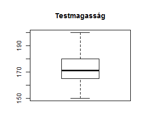
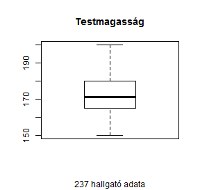
Alcím hozzáadása

boxplot(survey$Height, main="Testmagasság", sub="237 hallgató adata")

plot of chunk abrak_dobozdiagram_3

Az x tengely felirata

boxplot(survey$Height, main="Testmagasság", sub="237 hallgató adata", 
        xlab="University of Adelaide")

plot of chunk abrak_dobozdiagram_4

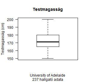
Az y tengely felirata

boxplot(survey$Height, main="Testmagasság", sub="237 hallgató adata", 
        xlab="University of Adelaide", ylab="Testmagasság (cm)")

plot of chunk abrak_dobozdiagram_5

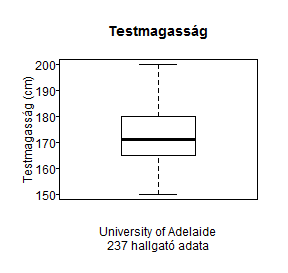
Tengelyfeliratok írásirányának megfordítása

par(las=1)
boxplot(survey$Height, main="Testmagasság", sub="237 hallgató adata", 
        xlab="University of Adelaide", ylab="Testmagasság (cm)")

plot of chunk abrak_dobozdiagram_6

Tengely és feliratok közelebb

par(las=1)
par(mgp=c(1.7, 0.2, 0))
boxplot(survey$Height, main="Testmagasság", sub="237 hallgató adata", 
        xlab="University of Adelaide", ylab="Testmagasság (cm)")

plot of chunk abrak_dobozdiagram_7

Léptekjel mérete és iránya

par(las=1)
par(mgp=c(1.7, 0.2, 0))
par(tcl=-0.2)
boxplot(survey$Height, main="Testmagasság", sub="237 hallgató adata", 
        xlab="University of Adelaide", ylab="Testmagasság (cm)")

plot of chunk abrak_dobozdiagram_8

Margók beállítása

par(las=1)
par(mgp=c(1.7, 0.2, 0))
par(tcl=-0.2)
par(mar=c(4.1, 3, 2, 1))
boxplot(survey$Height, main="Testmagasság", sub="237 hallgató adata", 
        xlab="University of Adelaide", ylab="Testmagasság (cm)")

plot of chunk abrak_dobozdiagram_9

Betűtípus beállítása

windowsFonts(Times="Times New Roman")
par(family = "Times")
par(las=1)
par(mgp=c(1.7, 0.2, 0))
par(tcl=-0.2)
par(mar=c(4.1, 3, 2, 1))
boxplot(survey$Height, main="Testmagasság", sub="237 hallgató adata", 
        xlab="University of Adelaide", ylab="Testmagasság (cm)")

plot of chunk abrak_dobozdiagram_10

Betűméret beállítása

windowsFonts(Times="Times New Roman")
par(family = "Times")
par(las=1)
par(mgp=c(1.7, 0.2, 0))
par(tcl=-0.2)
par(mar=c(4.1, 3, 2, 1))
boxplot(survey$Height, main="Testmagasság", sub="237 hallgató adata", 
        xlab="University of Adelaide", ylab="Testmagasság (cm)", 
        cex.main=1.4, cex.sub=1.1, cex.lab=1.1, cex.axis=0.8)

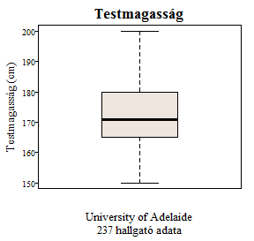
plot of chunk abrak_dobozdiagram_11

Dobozszínek beállítása

windowsFonts(Times="Times New Roman")
par(family = "Times")
par(las=1)
par(mgp=c(1.7, 0.2, 0))
par(tcl=-0.2)
par(mar=c(4.1, 3, 2, 1))
boxplot(survey$Height, main="Testmagasság", sub="237 hallgató adata", 
        xlab="University of Adelaide", ylab="Testmagasság (cm)", 
        cex.main=1.4, cex.sub=1.1, cex.lab=1.1, cex.axis=0.8, col="seashell2")

plot of chunk abrak_dobozdiagram_12

Ábra mentése

# png("kepek/kep_boxplot.png", width=1200, height=1200, res=300)
# windowsFonts(Times="Times New Roman")
# par(family = "Times")
# par(las=1)
# par(mgp=c(1.7, 0.2, 0))
# par(tcl=-0.2)
# par(mar=c(4.1, 3, 2, 1))
# boxplot(survey$Height, main="Testmagasság", sub="237 hallgató adata", xlab="University of Adelaide", ylab="Testmagasság (cm)", cex.main=1.4, cex.sub=1.1, cex.lab=1.1, cex.axis=0.8, col="seashell2") 
# dev.off()

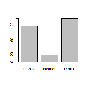
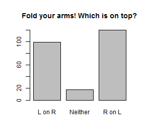
4. feladat. Oszlopdiagram.
Rajzoljunk oszlopdiagramot a MASS csomag survey adattáblájának Smoke változójára. Fokozatosan javítsuk, és tegyük publikációkésszé!

data(survey, package = "MASS") # a survey beolvasása
survey$Fold

  [1] R on L  R on L  L on R  R on L  Neither L on R  L on R  R on L  R on L  R on L  L on R 
 [12] R on L  L on R  L on R  R on L  R on L  L on R  R on L  L on R  R on L  R on L  L on R 
 [23] L on R  R on L  R on L  Neither R on L  R on L  L on R  L on R  R on L  L on R  R on L 
 [34] R on L  L on R  L on R  L on R  R on L  R on L  R on L  L on R  R on L  R on L  L on R 
 [45] L on R  R on L  L on R  R on L  R on L  R on L  R on L  L on R  L on R  L on R  R on L 
 [56] L on R  R on L  R on L  L on R  L on R  R on L  R on L  L on R  L on R  L on R  Neither
 [67] L on R  R on L  L on R  L on R  L on R  R on L  R on L  L on R  R on L  Neither L on R 
 [78] L on R  R on L  L on R  R on L  R on L  R on L  R on L  L on R  R on L  L on R  R on L 
 [89] Neither R on L  R on L  Neither L on R  R on L  R on L  L on R  R on L  R on L  Neither
[100] R on L  R on L  L on R  Neither R on L  R on L  R on L  R on L  R on L  L on R  R on L 
[111] R on L  L on R  R on L  R on L  L on R  L on R  R on L  L on R  L on R  L on R  R on L 
[122] L on R  R on L  L on R  L on R  R on L  R on L  L on R  R on L  L on R  R on L  L on R 
[133] R on L  L on R  R on L  L on R  L on R  L on R  L on R  L on R  R on L  R on L  R on L 
[144] L on R  R on L  R on L  L on R  R on L  L on R  R on L  R on L  L on R  L on R  R on L 
[155] L on R  R on L  L on R  L on R  R on L  L on R  R on L  Neither L on R  R on L  Neither
[166] R on L  R on L  L on R  L on R  R on L  L on R  L on R  Neither R on L  R on L  L on R 
[177] Neither L on R  R on L  R on L  R on L  R on L  L on R  L on R  Neither R on L  L on R 
[188] R on L  R on L  Neither R on L  L on R  R on L  L on R  Neither L on R  R on L  Neither
[199] R on L  R on L  R on L  L on R  R on L  Neither R on L  R on L  L on R  R on L  L on R 
[210] R on L  L on R  R on L  R on L  R on L  L on R  Neither L on R  R on L  L on R  L on R 
[221] L on R  R on L  R on L  L on R  L on R  R on L  R on L  L on R  L on R  L on R  R on L 
[232] R on L  L on R  L on R  R on L  R on L  R on L 
Levels: L on R Neither R on L

table(survey$Fold)


 L on R Neither  R on L 
     99      18     120

Kiinduló ábra

barplot(table(survey$Fold))

plot of chunk abrak_oszlopdiagram_1

Főcím hozzáadása

barplot(table(survey$Fold), main="Fold your arms! Which is on top?")

plot of chunk abrak_oszlopdiagram_2

Alcím hozzáadása

barplot(table(survey$Fold),  main="Fold your arms! Which is on top?", 
        sub="237 hallgató adata")

plot of chunk abrak_oszlopdiagram_3

Az x tengely felirata

barplot(table(survey$Fold), main="Fold your arms! Which is on top?", 
        sub="237 hallgató adata", xlab="University of Adelaide")

plot of chunk abrak_oszlopdiagram_4

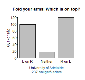
Az y tengely felirata

barplot(table(survey$Fold), main="Fold your arms! Which is on top?", 
        sub="237 hallgató adata", xlab="University of Adelaide", ylab="Gyakoriság")

plot of chunk abrak_oszlopdiagram_5

Tengelyfeliratok írásirányának megfordítása

par(las=1)
barplot(table(survey$Fold), main="Fold your arms! Which is on top?", 
        sub="237 hallgató adata", xlab="University of Adelaide", ylab="Gyakoriság")

plot of chunk abrak_oszlopdiagram_6

Tengely és feliratok közelebb

par(las=1)
par(mgp=c(1.7, 0.2, 0))
barplot(table(survey$Fold), main="Fold your arms! Which is on top?", 
        sub="237 hallgató adata", xlab="University of Adelaide", ylab="Gyakoriság")

plot of chunk abrak_oszlopdiagram_7

Léptekjel mérete és iránya

par(las=1)
par(mgp=c(1.7, 0.2, 0))
par(tcl=-0.2)
barplot(table(survey$Fold), main="Fold your arms! Which is on top?", 
        sub="237 hallgató adata", xlab="University of Adelaide", ylab="Gyakoriság")

plot of chunk abrak_oszlopdiagram_8

Margók beállítása

par(las=1)
par(mgp=c(1.7, 0.2, 0))
par(tcl=-0.2)
par(mar=c(4.1, 3, 2, 1))
barplot(table(survey$Fold), main="Fold your arms! Which is on top?", 
        sub="237 hallgató adata", xlab="University of Adelaide", ylab="Gyakoriság")

plot of chunk abrak_oszlopdiagram_9

Betűtípus beállítása

windowsFonts(Times="Times New Roman")
par(family = "Times")
par(las=1)
par(mgp=c(1.7, 0.2, 0))
par(tcl=-0.2)
par(mar=c(4.1, 3, 2, 1))
barplot(table(survey$Fold), main="Fold your arms! Which is on top?", 
        sub="237 hallgató adata", xlab="University of Adelaide", ylab="Gyakoriság")

plot of chunk abrak_oszlopdiagram_10

Betűméret beállítása

windowsFonts(Times="Times New Roman")
par(family = "Times")
par(las=1)
par(mgp=c(1.7, 0.2, 0))
par(tcl=-0.2)
par(mar=c(4.1, 3, 2, 1))
barplot(table(survey$Fold), main="Fold your arms! Which is on top?", 
        sub="237 hallgató adata", xlab="University of Adelaide", ylab="Gyakoriság",
        cex.main=1.4, cex.sub=1.1, cex.lab=1.1, cex.axis=0.8)

plot of chunk abrak_oszlopdiagram_11

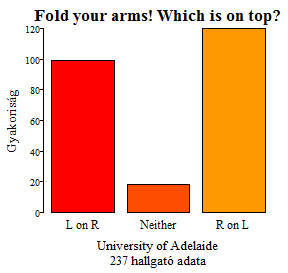
Oszlopszínek beállítása

windowsFonts(Times="Times New Roman")
par(family = "Times")
par(las=1)
par(mgp=c(1.7, 0.2, 0))
par(tcl=-0.2)
par(mar=c(4.1, 3, 2, 1))
barplot(table(survey$Fold), main="Fold your arms! Which is on top?", 
        sub="237 hallgató adata", xlab="University of Adelaide", ylab="Gyakoriság",
        cex.main=1.4, cex.sub=1.1, cex.lab=1.1, cex.axis=0.8, col=rainbow(20))

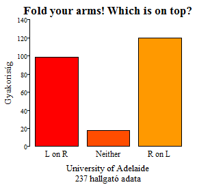
plot of chunk abrak_oszlopdiagram_12

Az y tengely láthatósági tartománya

windowsFonts(Times="Times New Roman")
par(family = "Times")
par(las=1)
par(mgp=c(1.7, 0.2, 0))
par(tcl=-0.2)
par(mar=c(4.1, 3, 2, 1))
barplot(table(survey$Fold), main="Fold your arms! Which is on top?", 
        sub="237 hallgató adata", xlab="University of Adelaide", ylab="Gyakoriság",
        cex.main=1.4, cex.sub=1.1, cex.lab=1.1, cex.axis=0.8, col=rainbow(20), ylim=c(0, 140))

plot of chunk abrak_oszlopdiagram_13

Ábra mentése

# png("kepek/kep_boxplot.png", width=1200, height=1200, res=300)
# windowsFonts(Times="Times New Roman")
# par(family = "Times")
# par(las=1)
# par(mgp=c(1.7, 0.2, 0))
# par(tcl=-0.2)
# par(mar=c(4.1, 3, 2, 1))
# barplot(table(survey$Fold), main="Fold your arms! Which is on top?", sub="237 hallgató adata", xlab="University of Adelaide", ylab="Gyakoriság", cex.main=1.4, cex.sub=1.1, cex.lab=1.1, cex.axis=0.8, col=rainbow(20), ylim=c(0, 140)) 
# dev.off()

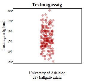
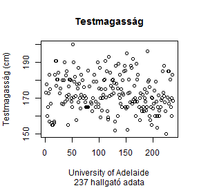
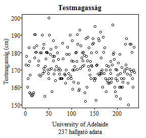
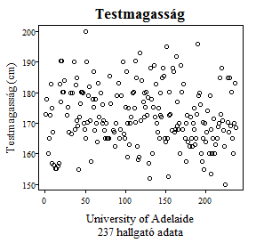
5. feladat. Szórásdiagram.
Rajzoljunk szórásdiagramot a MASS csomag survey adattáblájának Height változójára. Fokozatosan javítsuk, és tegyük publikációkésszé!

data(survey, package = "MASS") # a survey beolvasása
survey$Height

  [1] 173.00 177.80     NA 160.00 165.00 172.72 182.88 157.00 175.00 167.00 156.20     NA 155.00
 [14] 155.00     NA 156.00 157.00 182.88 190.50 177.00 190.50 180.34 180.34 184.00     NA     NA
 [27] 172.72 175.26     NA 167.00     NA 180.00 166.40 180.00     NA 190.00 168.00 182.50 185.00
 [40] 171.00 169.00 154.94 172.00 176.50 180.34 180.34 180.00 170.00 168.00 165.00 200.00 190.00
 [53] 170.18 179.00 182.00 171.00 157.48     NA 177.80 175.26 187.00 167.64 178.00 170.00 164.00
 [66] 183.00 172.00     NA 180.00     NA 170.00 176.00 171.00 167.64 165.00 170.00 165.00 165.10
 [79] 165.10 185.42     NA 176.50     NA     NA 167.64 167.00 162.56 170.00 179.00     NA 183.00
 [92]     NA 165.00 168.00 179.00     NA 190.00 166.50 165.00 175.26 187.00 170.00 159.00 175.00
[105] 163.00 170.00 172.00     NA 180.00 180.34 175.00 190.50 170.18 185.00 162.56 158.00 159.00
[118] 193.04 171.00 184.00     NA 177.00 172.00 180.00 175.26 180.34 172.72 178.50 157.00 152.00
[131] 187.96 178.00     NA 160.02 175.26 189.00 172.00 182.88 170.00 167.00 175.00 165.00 172.72
[144] 180.00 172.00 185.00 187.96 185.42 165.00 164.00 195.00 165.00 152.40 172.72 180.34 173.00
[157]     NA 167.64 187.96 187.00 167.00 168.00 191.80 169.20 177.00 168.00 170.00 160.02 189.00
[170] 180.34 168.00 182.88     NA 165.00 157.48 170.00 172.72 164.00     NA 162.56 172.00 165.10
[183] 162.50 170.00 175.00 168.00 163.00 165.00 173.00 196.00 179.10 180.00 176.00 160.02 157.48
[196] 165.00 170.18 154.94 170.00 164.00 167.00 174.00     NA 160.00 179.10 168.00 153.50 160.00
[209] 165.00 171.50 160.00 163.00     NA 165.00 168.90 170.00     NA 185.00 173.00 188.00 171.00
[222] 167.64 162.56 150.00     NA     NA 170.18 185.00 167.00 185.00 169.00 180.34 165.10 160.00
[235] 170.00 183.00 168.50

Kiinduló ábra

plot(survey$Height)

plot of chunk abrak_ketdimpont_1

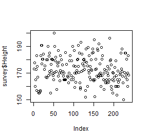
Főcím hozzáadása

plot(survey$Height, main="Testmagasság")

plot of chunk abrak_ketdimpont_2

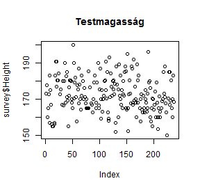
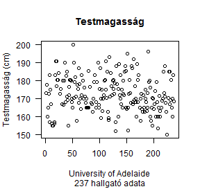
Alcím hozzáadása

plot(survey$Height,  main="Testmagasság", sub="237 hallgató adata")

plot of chunk abrak_ketdimpont_3

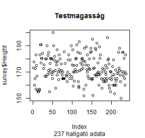
Az x tengely felirata

plot(survey$Height, main="Testmagasság", sub="237 hallgató adata", 
     xlab="University of Adelaide")

plot of chunk abrak_ketdimpont_4

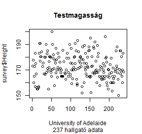
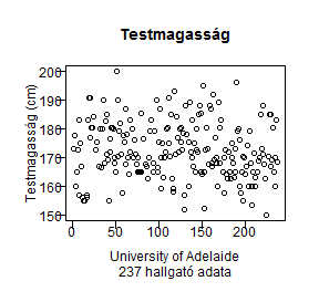
Az y tengely felirata

plot(survey$Height, main="Testmagasság", sub="237 hallgató adata", 
     xlab="University of Adelaide", ylab="Testmagasság (cm)")

plot of chunk abrak_ketdimpont_5

Tengelyfeliratok írásirányának megfordítása

par(las=1)
plot(survey$Height, main="Testmagasság", sub="237 hallgató adata", 
     xlab="University of Adelaide", ylab="Testmagasság (cm)")

plot of chunk abrak_ketdimpont_6

Tengely és feliratok közelebb

par(las=1)
par(mgp=c(1.7, 0.2, 0))
plot(survey$Height, main="Testmagasság", sub="237 hallgató adata", 
     xlab="University of Adelaide", ylab="Testmagasság (cm)")

plot of chunk abrak_ketdimpont_7

Léptekjel mérete és iránya

par(las=1)
par(mgp=c(1.7, 0.2, 0))
par(tcl=-0.2)
plot(survey$Height, main="Testmagasság", sub="237 hallgató adata", 
     xlab="University of Adelaide", ylab="Testmagasság (cm)")

plot of chunk abrak_ketdimpont_8

Margók beállítása

par(las=1)
par(mgp=c(1.7, 0.2, 0))
par(tcl=-0.2)
par(mar=c(4.1, 3, 2, 1))
plot(survey$Height, main="Testmagasság", sub="237 hallgató adata", 
     xlab="University of Adelaide", ylab="Testmagasság (cm)")

plot of chunk abrak_ketdimpont_9

Betűtípus beállítása

windowsFonts(Times="Times New Roman")
par(family = "Times")
par(las=1)
par(mgp=c(1.7, 0.2, 0))
par(tcl=-0.2)
par(mar=c(4.1, 3, 2, 1))
plot(survey$Height, main="Testmagasság", sub="237 hallgató adata", 
     xlab="University of Adelaide", ylab="Testmagasság (cm)")

plot of chunk abrak_ketdimpont_10

Betűméret beállítása

windowsFonts(Times="Times New Roman")
par(family = "Times")
par(las=1)
par(mgp=c(1.7, 0.2, 0))
par(tcl=-0.2)
par(mar=c(4.1, 3, 2, 1))
plot(survey$Height, main="Testmagasság", sub="237 hallgató adata", 
     xlab="University of Adelaide", ylab="Testmagasság (cm)", 
     cex.main=1.4, cex.sub=1.1, cex.lab=1.1, cex.axis=0.8)

plot of chunk abrak_ketdimpont_11

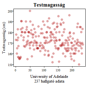
Pontkarakter beállítása: alak és szín

windowsFonts(Times="Times New Roman")
par(family = "Times")
par(las=1)
par(mgp=c(1.7, 0.2, 0))
par(tcl=-0.2)
par(mar=c(4.1, 3, 2, 1))
plot(survey$Height, main="Testmagasság", sub="237 hallgató adata", 
     xlab="University of Adelaide", ylab="Testmagasság (cm)", 
     cex.main=1.4, cex.sub=1.1, cex.lab=1.1, cex.axis=0.8, 
     pch=21, col="#aa000010", bg="#aa000055", cex=1.5)

plot of chunk abrak_ketdimpont_12

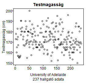
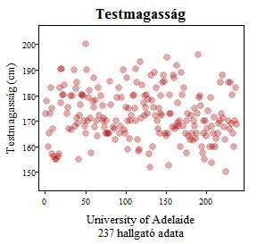
Az x és y tengely láthatósági tartománya

windowsFonts(Times="Times New Roman")
par(family = "Times")
par(las=1)
par(mgp=c(1.7, 0.2, 0))
par(tcl=-0.2)
par(mar=c(4.1, 3, 2, 1))
plot(survey$Height, main="Testmagasság", sub="237 hallgató adata", 
     xlab="University of Adelaide", ylab="Testmagasság (cm)", 
     cex.main=1.4, cex.sub=1.1, cex.lab=1.1, cex.axis=0.8, 
     pch=21, col="#aa000010", bg="#aa000055", cex=1.5, ylim=c(145, 205))

plot of chunk abrak_ketdimpont_13

Ábra mentése

# png("kepek/kep_boxplot.png", width=1200, height=1200, res=300)
# windowsFonts(Times="Times New Roman")
# par(family = "Times")
# par(las=1)
# par(mgp=c(1.7, 0.2, 0))
# par(tcl=-0.2)
# par(mar=c(4.1, 3, 2, 1))
# plot(survey$Height, main="Testmagasság", sub="237 hallgató adata", xlab="University of Adelaide", ylab="Testmagasság (cm)", cex.main=1.4, cex.sub=1.1, cex.lab=1.1, cex.axis=0.8, pch=21, col="#aa000010", bg="#aa000055", cex=1.5, ylim=c(145, 205)) 
# dev.off()