4 Item response theory

Item response theory (IRT; e.g. Embretson & Reise, 2000), or latent trait theory (e.g., Borsboom 2008) is a newer approach applied in test construction and evaluation. In contrast with classical test theory where the emphasis is on the test as a whole entity, and the characteristics (e.g. reliability, validity) of the test, in IRT the focus is on the smallest unit of the test, the item, and the characteristics, parameters are estimated by fitting models on the data. IRT originally was used primarily for ability tests, where a correct answer could be defined, like for example in multiple choice tests. Hence, the first IRT models were meant for such correct/incorrect dichotomous items. Although IRT models can also be applied for constructs that cannot be termed as abilities, for example attitudes, personality characteristics, etc. we will use “ability” to denote the underlying construct. The terms correct and incorrect answers will also be used even if there are cases when there is no correct answer.

In IRT the aim is to estimate the parameters (characteristics) of the items, and use this information to construct tests to estimate the test taker’s ability. A major advantage of IRT that based on its principles it is possible to establish item banks consisting of hundreds or thousands of questions, and then appropriately choosing from this pool one can create tailor made tests, that perfectly fit for the purpose and target population of the testing. It is also possible to use computer adaptive testing, where after each item it is possible to update the estimate of the test taker’s ability, and pick the next item taking this estimate into account. This way of proceeding makes it possible to get a reliable estimate of the ability using relatively few items.

4.1 IRT models for dichotomous variables

The simplest IRT model is the one parameter logistic model (1PL; Rasch, 1960). In this model the probability of the correct answer depends on the ability of the test taker, and the difficulty of the item.

\[P(x=1|\theta_p,\beta_i)=\frac{e^{(\theta_p-\beta_i)}}{1+e^{(\theta_p-\beta_i)}}\]

where θ_p is the ability paramerter of person p and β_i is the difficulty parameter of item i. Plotting the above function result in the item characteristic curve (ICC) a basic concept in IRT. In Figure 3 an example ICC is plotted.

The difficulty parameter is defined with the ability that is necessary to have probability of .5 to correctly answer the item, or stated in other words, the difficulty of an item equals the ability, with which half the test takers answer correctly. The difficulty parameter of the item in Figure 3. can easily be seen with the help of the dashed lines. The difficulty parameter of this item is 0. Under the 1PL model the ICCs of the items are identical, only the location (difficulty) may be different among the items.

If not only the location but, the slope (discrimination) of the ICCs may be different across the items we get the two parameter logistic model (2PL) where the item specific discrimination (slope) parameter, α_i is also part of the model (Birnbaum, 1968).

\[P(x=1|\theta_p,\beta_i, \alpha_i)=\frac{e^{\alpha_i(\theta_p-\beta_i)}}{1+e^{\alpha_i(\theta_p-\beta_i)}}\]

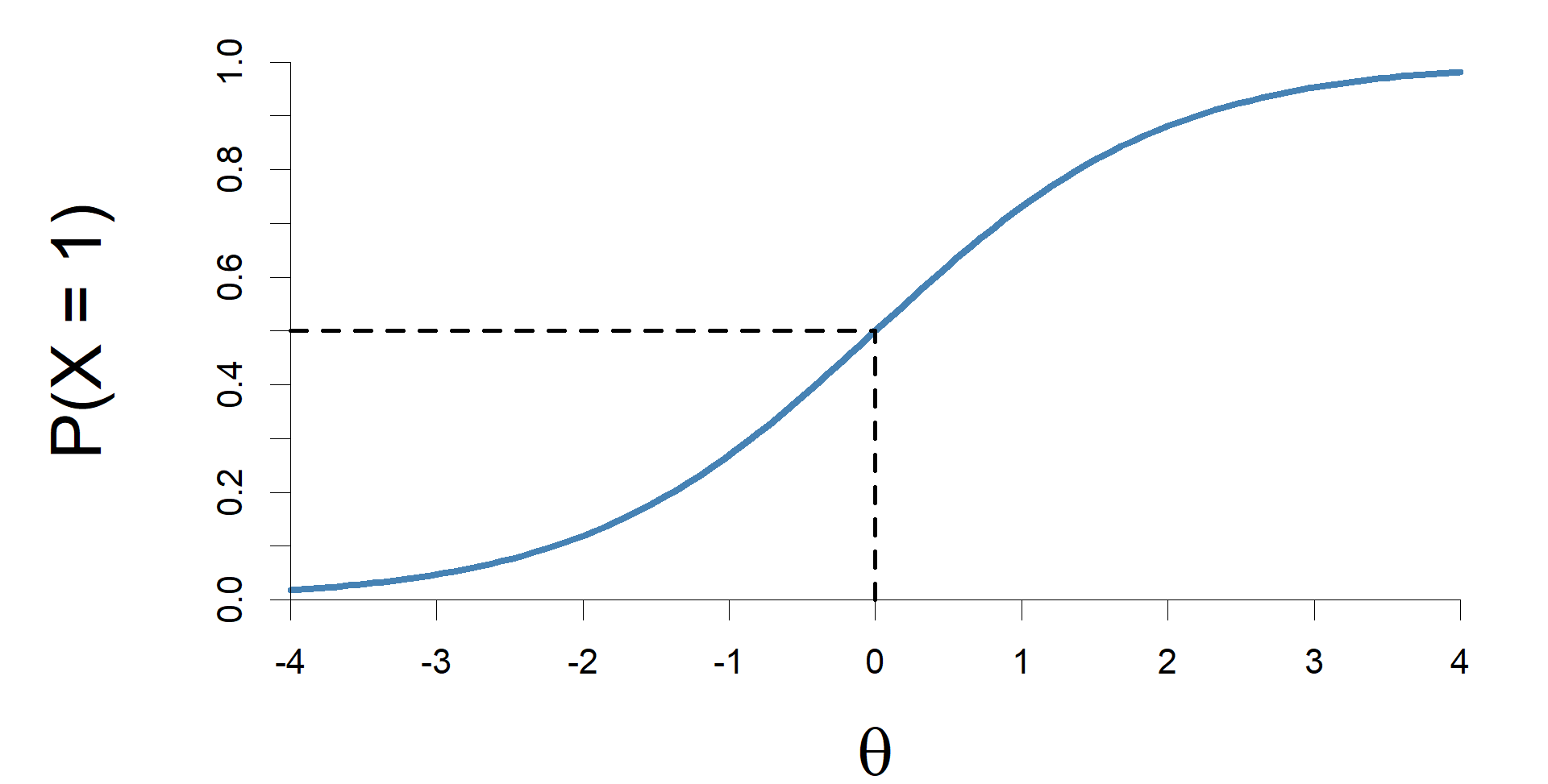
Figure 3. The item characteristic curve of an item under the one parameter logistic model.

It is important to note that a higher value of the discrimination parameter means a higher discrimination, that is the item discriminate better between test takers with higher and lower ability, but it only holds in the region around the difficulty parameter of the item, otherwise the discriminative power of the item may be weaker than in case of an item with a smaller discrimination parameter.

The 1PL and 2PL models assume that when the ability is very low the probability of a correct answer converge to zero. However, this assumption is not always feasible, as it may happen in case of a multiple choice item, for example, that the probability of a correct answer is significantly different from zero even if the ability is infinitely low. The three parameter logistic model (3PL; Birnbaum, 1968) takes this possibility into account by including a guessing parameter γ_i.

\[P(x=1|\theta_p,\beta_i, \alpha_i, \gamma_i)=\gamma_i+(1-\gamma_i)\frac{e^{\alpha_i(\theta_p-\beta_i)}}{1+e^{\alpha_i(\theta_p-\beta_i)}}\]

The ICC of an item under the 3PL model is depicted in Figure 4.

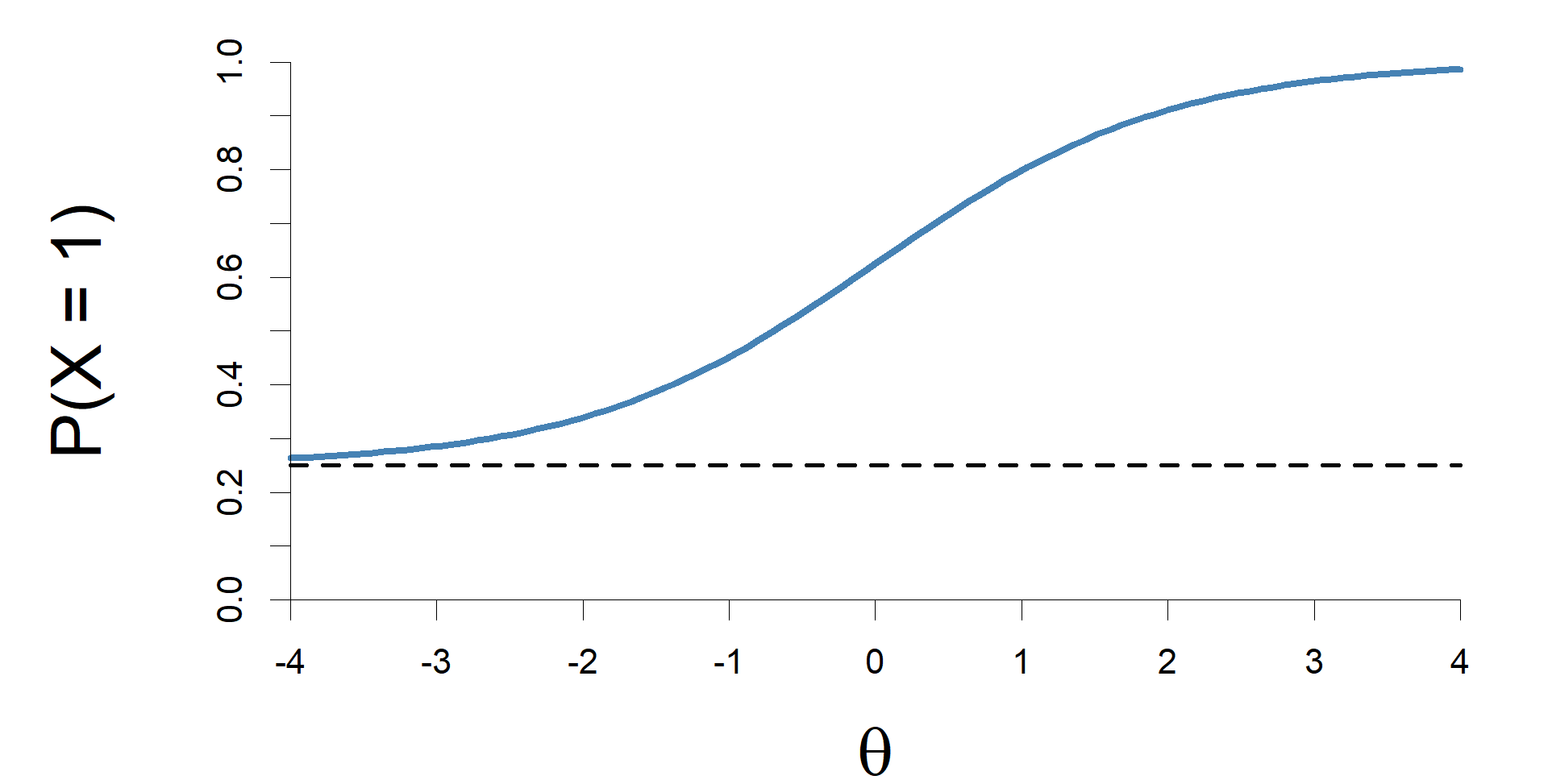
Figure 4. The item characteristic curve of an item under the three parameter logistic model, with a guessing parameter of .25.

4.2 IRT models for polytomous variables

Beyond the models for dichotomous data described above, IRT models for polytomous data are also available. As mentioned above IRT models originally were used in performance tests using dichotomous data, but many times there is a need for such models when for the items do not only have correct or incorrect answer, but credit may be obtained for example when part of the solution is correct. Another example may be when the items are scored on a scale, like in case of the depression measure described above, where the respondent is to indicate how often s/he experienced the phenomenon in the statement on a four-point (0-3) scale. To address the need to anlyze and interpret such data several models were proposed. The more popular of these are the Rating Scale Model (Andrich, 1978), the Partial Credit Model (Masters, 1982), and the Graded Response Model (GRM; Samejima, 1969), of which the latter is to be presented briefly. GRM can be considered as a generalization of the 2PL model (see above) for polytomous data, measured on an ordinal scale. The rationale for this generalization is the dichotomization of the polytomous variable. The polytomous variable can be transformed to a dichotomous one in k-1 ways, k being the number of response options, and for these dichotomous variables the 2PL model can be applied.

\[P(x\geq k|\theta_p,\beta_{ik}, \alpha_i)=\frac{e^{\alpha_i(\theta_p-\beta_{ik})}}{1+e^{\alpha_i(\theta_p-\beta_{ik})}}\]

where k is the k^th response category of the item, β_ik is the k^th threshold, that is, the threshold for category k. This way, not the probability of responding in a certain category but rather, the probability of responding in a certain category or higher is modeled. The probability of responding in a given category obtained by

\[ P(x= k|\theta_p,\beta_{ik}, \alpha_i)=P(x\geq k|\theta_p,\beta_{ik}, \alpha_i)-P(x\geq k+1|\theta_p,\beta_{ik+1}, \alpha_i) \]

except for the highest response category, where

\[ P(x= k|\theta_p,\beta_{ik}, \alpha_i)=P(x\geq k|\theta_p,\beta_{ik}, \alpha_i) \]