3 Classical test theory

In classical test theory, the basic assumption is that the construct in question can in fact be measured, and that the construct has a given value for the subject of measurement, that is, it has a true score, and the goal of the measurement is to find that true score value. (That is why classical test theory is often called true score theory.) As this true score is never known with absolute confidence, the measured value (the result of the measurement) can be defined as the true score plus an error term, as presumably the measurement process is not perfect. This is the basic equation of classical test theory.

\[X = T + \epsilon\]

where X is the empirically observed test score, T is the True score value and ε is the error component.

The error of the measurement can be of two types. Systematic error, or bias occurs when the measurement results are systematically biased, that is, the error of the measurement is not random. It may happen for example when a short-sighted person takes the test without using appropriate glasses, and hence not able to properly read the instructions, or properly perceive test stimuli. The test result in such cases will tend to be lower than the true score of the test taker. Unsystematic bias, on the other hand is such that it is random, that is, the expected value of the measurement equals exactly the true score.

Classical test theory is built on a few axioms (e.g., Münnich et al., 2002).

\[\epsilon \sim N(0, \sigma)\]

The error of the measurement follows a normal distribution with zero mean\[ \rho_{T\epsilon}=0 \]

The error of the measurement is independent of the true score\[ \rho_{\epsilon\epsilon'}=0 \] The error of the independent measurements are also independent of one another

3.1 Reliability

One of the key characteristics of a test in classical test theory is the reliability of the measurement instrument. Reliability is most commonly referenced by test-retest reliability that expresses the correlation between the results of the measurement at two different time points. This correlation is obviously expected to be positive, and the closer it is to 1 the more reliable the measurement instrument is considered. However, the repeated test administration with the same test takers, under the same conditions is practically not possible, and rather expensive, hence, other solutions were highly needed to address this question.

One such solution might be the split-half method to find an estimate of reliability (Brown, 1910; Spearman, 1910). The essence of the method, that the measurement instrument may be split into two halves, the scale score calculated for both halves and the correlation between the scale score may be calculated. This is an internal consistency approach of the reliability issue. However, the way an instrument split in halves is arbitrary, and hence the correlation of the resulting scale score of the halves may be quite different depending on the split. A possible solution for this problem may be to take all possible splits, calculate the correlations and finally calculate the mean of these correlations and use it as a measure of internal consistency. But obviously, this is a very time-consuming effort to find a reliability measure.

To overcome the problems of test-retest and split-half methods several coefficients were proposed to be used as reliability measures. One of the most well-known such coefficients is the KR20 formula (Kuder & Richardson, 1937), which was the basis for the alpha-coefficient proposed by Cronbach (1951). Cronbach’s alpha coefficient is still the most well-known, broadly accepted, and most frequently applied measure of internal consistency, that is implemented in standard statistical software packages. Cornbach’s alpha can be calculated as follows:

\[\alpha=\frac{I}{I-1}\Big(1-\frac{\sum_{i=1}^{I}var(x_i)}{var(X)}\Big)\]

where I is the number of items, x_i is the i^thitem, and X is the total score on the test.

In spite of the unquestionable popularity of Cronbach’s alpha it has to be noted, that there are also potential problems when using this consistency coefficient. One such caveat is that the value of the reliability and hence that of the alpha coefficient is dependent on the number of the items, the more items are present in a scale, the higher the reliability. This has been recognized already by Brown (1910) and Spearman (1910), who created the following formula to account for this phenomenon:

\[rel(X_{ntimes}) =\frac{n rel(X)}{1+(n-1)rel(X)}\]

The Spearman-Brown formula can be used to estimate reliability using the split-half method, under the assumption that the test halves can be considered to be parallel tests, that measure the same underlying construct in the same way. The value of coefficient alpha is also dependent on the scale of the variables, which adds to the problem of interpreting the reliability based on alpha, as the acceptable value of alpha may be different in case of different variable scales and tests of different lengths. In general, the required value of the alpha coefficient is at least .8, but values above .7 are considered to be acceptable already. In principle the closer the value to one the better the reliability, that is true, but in practice a too high alpha value may also pose a problem, as it means that the items practically measure the exact same content, and hence one item would measure the underlying construct equally well as compared to the longer test. (Münnich et al., 2002)

Another problem when using Cronbach’s alpha is that an acceptably large alpha is often considered as a proof that the measure is unidimensional (measures one single underlying construct), but it is not always the case. A high alpha might be obtained even when the measurement instrument measure different underlying latent constructs.

To evaluate the dimensionality of the measurement instrument most typically principal components analysis, and factor analysis is applied (see below the scale construction section).

In order to demonstrate how can one compute certain characteristics of classical test theory in R a data set containing the responses of 79 test takers to 16 items of the Center for Epidemiologic Studies Depression Scale shall be used. (The original scale consists of 20 items, but the reverse-keyed (positively-keyed) items are left out of this data set.)

The 16 items of the data set are scored from 0 to 3, higher numbers indicating more frequent occurrence of the phenomenon stated in the item.

The first six rows of the data set looks like this:

head(df)

##   V1 V2 V3 V4 V5 V6 V7 V8 V9 V10 V11 V12 V13 V14 V15 V16
## 1  3  3  3  3  3  3  3  3  3   3   3   3   3   3   3   3
## 2  2  1  2  2  2  2  3  2  2   1   1   1   0   2   1   1
## 3  2  0  2  2  2  2  1  1  1   1   0   0   1   2   1   2
## 4  2  3  2  2  3  1  0  1  1   2   2   0   2   2   1   2
## 5  2  0  1  1  2  2  1  1  0   1   1   1   1   1   1   1
## 6  2  2  2  2  3  3  3  2  2   1   1   2   2   3   3   3

To obtain the Cronbach’s alpha coefficient the reliability function of the RcmdrMisc R package (Fox, 2020) may be used.

RcmdrMisc::reliability(cov(df))$alpha

##     alpha 
## 0.8370298

As can be seen the Cronbach’s alpha coefficient is relatively large at .84, suggesting that this 16-item scale is a reliable measure of depression.

3.1.1 Standard error of measurement in classical test

theory {.unnumbered}

In classical test theory the standard error of measurement can be calculated using the reliability of the applied measurement instrument and the standard deviation of the total scores of the scale:

\[SE=\sigma X * \sqrt{(1-\alpha)} \]

In case of our depression measure the standard error of measurement can be calculated as follows:

total <- rowSums(df) # calcuting the total score
sigma <- sd(total)   # standard deviation of the total 
alpha <- RcmdrMisc::reliability(cov(df))$alpha # calcuting reliability

SE <- sigma*sqrt(1-alpha)
SE

##    alpha 
## 3.413832

That is, the standard error of measurement for the 16-item depression measure is 3.41. Given this value one can calculate a confidence interval for the estimate of the depression value. For a total score of 20, for example, the 95% confidence interval can be calculated like:

CI1 <- 20 -1.96*SE  # a 95%-os konfidencia intervallum alsó végpontja
CI2 <- 20 + 1.96*SE # a 95%-os konfidencia intervallum felső végpontja
CI1

##    alpha 
## 13.30889

CI2

##    alpha 
## 26.69111

3.2 Validity

Besides the reliability construct the other very prominent characteristic of a test based on classical test theory is that of the validity of the test. While reliability expresses how well we measure the construct in question, validity refer to what extent we measure the very thing we aim to measure.

Most of the time, the way to corroborate that a certain measure is an acceptable measure of a construct is to find a characteristic that can be accepted as measuring the exact same, or maybe similar thing, and establish a connection with that construct. Correlation is a naturally occurring measure to establish the connection and the validity of our measure hence obtained.

Let’s suppose, for example, that one wants to measure intelligence, and constructs (see later) a measurement instrument to do so. When this instrument is ready one can look for a measure that must be connected to intelligence. This can be something like performance in school, which is, at least to a certain extent supposed to be determined by intelligence (and many other determinants as well). So what one can do is to calculate the results of the constructed scale, and correlate this result with the average school grades to verify the validity of the constructed scale.

This type of validity is commonly called criterion validity, as a criterion (average school grade in this example) is used to validate the scale. This characteristic of the classical test theory is based on correlation similar to the reliability construct.

3.3 Scale construction

In classical test theory principal components analysis (PCA; e.g. Münnich, Nagy & Abari, 2006) is often used to support scale construction. One advantage of this procedure is that unidimensionality of the data can be checked as it is a common assumption that the test or scale measure a single underlying construct. Another advantage of the method, that a weighted sum of the items can be calculated, taking the importance of the items into account, and hence a more appropriate measure can be used (Münnich et al., 2001).

PCA is a mathematical procedure aimed to extract information of several variables. As a result of the procedure of the I correlated initial variables I uncorrelated variables, so called principal components are calculated. The k^th principal component can be calculated as follows:

\[PC_k = w_{1k}X_1+w_{2k}X_2+w_{3k}X_3+ ... +w_{Ik}X_{I}\]

where PC_k is the kth principal component, w_ik is the weight of the ith item in case the k^th principal component and X_i is the ith original variable.

The item weights w_ik are chosen such that the resulting principal component has variance as large as possible. As this assumption alone would imply increasing the item weights to infinity a constraint has to be applied on these weights, such that

\[ \sum_{i=1}^{I}{w_{ik}^2}=1 \]

that is, the sum of squared weights should be equal to one, for every principal component.

When calculating the weights of the original variables to obtain the principal components, it is important to weigh the variables in a way that the resulting principal component is independent of all the other principal components, that is their correlation is zero, hence the principal components represent independent sources of the information represented by the original variables.

When the principal components are calculated one is to check how many principal components are of interest. One method to do that is to plot the variance of the principal components and find the one which has a large drop in variance. This method is called the scree method. The other method is find the principal components having a variance above one, if using a correlation matrix input. The rationale of this method is that the variance of a single observed standardized variable is one (that will be the case when PCA is performed on the correction matrix of the variables, or the covariance matrix of the standardized variables), so any principal components with variance below one has less information than a single observed variable.

In R there are several possible ways to perform PCA of which here the princomp function of the stats package (R Core Team, 2021) is used.

# perform principal components analysis on the variables of df data frame
p.c.a <- princomp(df, cor = TRUE) 

# plot the variances of the resulting principal components
barplot(p.c.a$sdev^2, col = "steelblue", las = 2)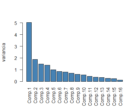

Figure 1. Barplot of the variances of the principal components

Using the scree method on the barplot in Figure 1., one could conclude that this 16-item measure of depression can be considered to be unidimensional, as there is a huge drop in variance after the first principal component. However, taking the absolute values of the principal components into account, one could conclude that the 16-item measure must be four-dimensional, as the number of principal components with variance larger than one is four. Taking into account that the 16 items measure four facets of depression symptoms this empirical result seems to be in line with theory.

The results of the PCA can be used for further purposes as well, beyond investigating the dimensionality of the measurement instrument. One such use of the results can be to use the principal components weights to calculate a principal component score as a weighted score, hence creating a measure of the dimension in focus that incorporates the importance of the items of the scale. It is important to note that, because of the characteristics of the algorithm, the weighted scale may be reversed as compared to the original scale, that is important be checked.

# creating a weighted scale score (wss) in the original data set
df$wss <- round(p.c.a$scores[, 1], 2)

# the first six rows of the data frame 
head(df)

##   V1 V2 V3 V4 V5 V6 V7 V8 V9 V10 V11 V12 V13 V14 V15 V16   wss
## 1  3  3  3  3  3  3  3  3  3   3   3   3   3   3   3   3  5.51
## 2  2  1  2  2  2  2  3  2  2   1   1   1   0   2   1   1  0.09
## 3  2  0  2  2  2  2  1  1  1   1   0   0   1   2   1   2 -0.96
## 4  2  3  2  2  3  1  0  1  1   2   2   0   2   2   1   2  0.04
## 5  2  0  1  1  2  2  1  1  0   1   1   1   1   1   1   1 -1.80
## 6  2  2  2  2  3  3  3  2  2   1   1   2   2   3   3   3  2.98

Another use of the PCA results is to calculate a reliability measure based on the loading of the first principal component.

\[ \theta = \frac{I}{I-1}(1-\frac{1}{\lambda_1}) \]

where I is the number of items and \(\lambda_i\) is the loading of the first principal component.

The θ reliability coefficient is a better approximation of the true reliability of the scale compared to Cronbach’s α coefficient which is a lower estimation of the reliability. In contrast with the α coefficient, θ reliability coefficient can also corroborate unidimensionality.

# calculating the theta reliability coefficient
nitems <- 16
theta <- (nitems/(nitems-1)) * (1 - 1/p.c.a$sdev[1]^2)
theta

##    Comp.1 
## 0.8546059

3.4 Test score interpretation

When using tests to measure psychological constructs interpretation of the test results is a crucial question.

The sum score of the test, as a raw score may be informative in some cases, for example when it expresses the number of tasks correctly solved, and this may be the basis for the evaluation of the test takers’ ability or performance. This kind of interpretation can be established by expert opinion, for example. Many times it is possible to find threshold values, standards of performance, that can be considered as a minimum requirement to pass an exam, for instance. In case this threshold performance is not reached, passing the exam is not possible, and it holds even if all the test takers fail. (Although such a case would raise serious questions regarding the adequacy of the test, and/or the quality of the teaching of the material tested.) (Cronbach, 1990.)

However, the absolute value of the correct answers is not necessarily informative when one wants to place the test taker in a population. In such cases a standard, or norm sample is to be used to compare the result of a test taker. Norm-referenced interpretation is widely used and has the advantage that relative performance can be used if there are no clearly defined performance standards for the construct.

When using norm-referenced interpretation of test scores there are several methods to transform the raw test scores in order to assign a value to test takers that expresses their position relative to the norm sample. One of these methods is the well-known standardization of the data, where the transformed values of the raw scores are z scores, obtained by subtracting the mean of the raw scores from a test taker’s raw score and then dividing it by the standard deviation of the raw scores. The z scores are relatively easy to interpret as these are values from a standard normal distribution (z ~ N(0, 1) ). Another popular method to transform the raw scores on a test is to transform these to T values. This transformation is based on the above described standardization, but here the values are projected to a normal distribution with a mean of 50 and a standard deviation of 10. A similar procedure is used for IQ scores in many cases, where the raw test scores are projected on a normal distribution with a mean of 100 and standard deviation of 15. These methods assume that the test scores follow a normal distribution in the population.

Using percentile values is also a popular norm-referenced interpretation of the test scores. Percentiles are obtained by calculating what proportion of the members of the norm sample reach a certain score or lower. (If there are more than one members of the norm sample with this specific score half of them considered to have the score or lower.) This is a fairly intuitive method that is very easy to interpret, and also not sensitive to violations of the normality of the data. Yet another way to transform the raw test scores into more interpretable ones is to use the standard nine (ST9; stanine) scale. This transformation is based on z scores as well. ST9 values are obtained by dividing the z scores into intervals of 0.5 standard deviation, as can be seen on Figure 2. The percentile values in the intervals show the approximate proportion of the population falling into the given ST9 category.

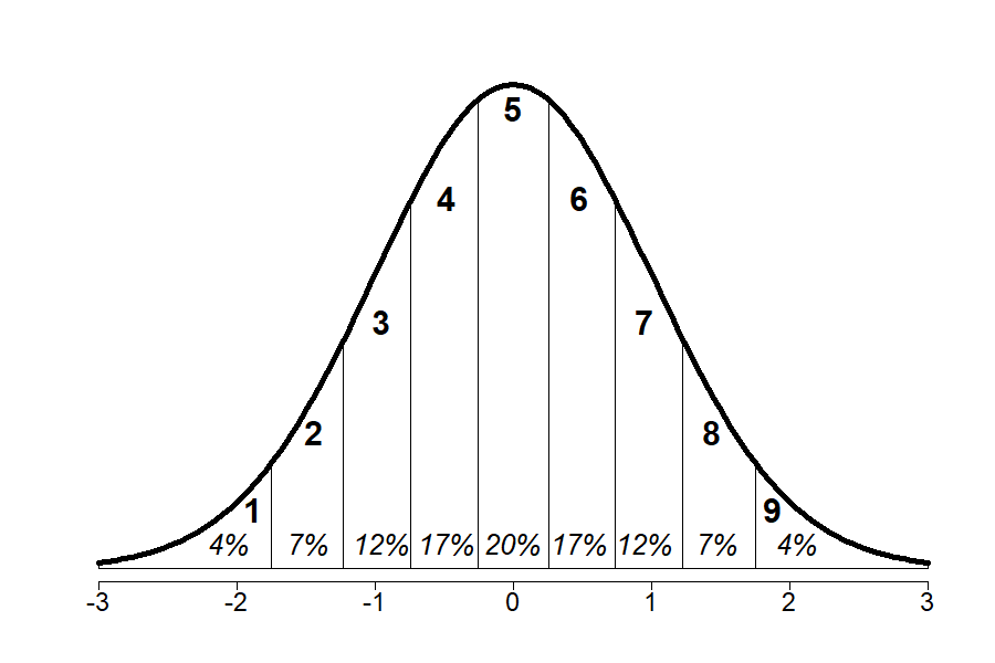
Figure 2. The Standard Nine scale with the proportion of the values

As can be seen all these transformations of the raw scores aim to help the test user to place the test taker relative to the population, or at least relative to the norm sample used as a reference. It is important to note that the above transformations, except for the percentiles, assume normally distributed data, that is a feasible assumption in many, but not all the cases. When the raw test scores are not normally distributed, for example skewed it is possible to transform the distribution of the data to normal distribution. The way to obtain these normalized scores is to calculate the empirical cumulative probability for each raw score of the test, and then find the value of a normal (most likely standard normal) distribution which has the same cumulative probability in that normal distribution. Transforming the raw scores to the corresponding value from the normal distribution shall result in a normally distributed variable. If the standard normal distribution is applied to implement the normalization than normalized standard scores are obtained. It is important to keep in mind, however, that normalization has been applied, because in some cases it is of high importance to take that into account when interpreting the results.

3.5 Test equating

It is not infrequent that testing involves more than one version of a test that aim at measuring the very same underlying construct. The most common reason to create more than one version is to avoid biased results due to the fact that when using a test the items may become known for those who take the test at a later occasion, or when it is necessary to retest the test takers after some time. Using alternative versions of the same test seems to be a good practice to avoid undue advantages. However, appealing as it is, alternative versions of a test may pose some difficulties when it comes to interpreting test results and comparing them across test versions. The reason is that, even if the test versions are prepared to be as equivalent in content and difficulty as possible, it is hardly possible to establish perfectly equivalent versions. Here comes test equating into play, that is one has to establish a connection between the test versions, giving which test score of version A is equivalent to which test score of version B. Two test scores stemming from different versions of the same test can be considered to be equivalent if the test takers obtaining those scores take the exact same position in the population.

In classical test theory there are two popular methods to establish the equivalence. The first method is called linear equating. This method is based on the standardization of the test score of version A in question and then finding the test score on version B that has the same z score.

\[ \frac{x_A-\mu_A}{\sigma_A}=\frac{x_B-\mu_B}{\sigma_B} \]

where x_A is the test score of version A for which the equivalent value is the question, µ_A is the mean of test scores for version A, σ_A is the standard deviation of the test score for version A. The symbols with subscript B are the corresponding values for version B. From the equation above the x_B value can be calculated as follows:

\[ x_B=\frac{x_A-\mu_A}{\sigma_A}\sigma_B+\mu_B \]

The other popular method is called equipercentile equating, and as the name suggest it is based on the calculation of percentiles. As follows from the calculation method of the percentiles, a test score from version A is equivalent with a test score from version B if both have the same percentile value.

In order to perform test equating different study designs may be applied. One natural choice may be a between-subject design where the subjects are randomly assigned to one of two groups (given that there are two versions of the test to be compared). One of the groups take test version A, while the other take test version B. As long as given a sufficiently large sample and the subjects are assigned randomly one can assume that the two groups can be considered equivalent. And if the equivalence of the groups are ensured, the potential differences of the test results may only stem from the differences of the test versions, and test equating can be implemented. A second approach to address the problem of equivalent groups is to apply a within-subject design, where the subjects are assigned to more than one experimental conditions, that is, in case of two groups (two test versions) all the subjects take both test versions. This way of proceeding ensures that the groups taking the versions of the test are equivalent as these consist of the same subjects. However, in case of a within-subject design problems may occur as well. The most likely problem is the order effect, that is, the order in which the test versions are taken may have an effect on the results of the test versions. To avoid this problem one may use some kind of balancing, for example the subjects are randomly assigned to groups, and one of the groups take version A followed by version B, whereas the other group take version B first, and then version A. Other solutions are also possible, like for example just mixing the items of the different versions, etc.